你现在手里有一份大小为 n x n 的 网格 grid,上面的每个 单元格 都用 0 和 1 标记好了。其中 0 代表海洋,1
请你找出一个海洋单元格,这个海洋单元格到离它最近的陆地单元格的距离是最大的,并返回该距离。如果网格上只有陆地或者海洋,请返回 -1。
我们这里说的距离是「曼哈顿距离」( Manhattan Distance):(x0, y0) 和 (x1, y1) 这两个单元格之间的距离是|x0 - x1| + |y0 - y1| 。
示例 1:
 和所有陆地单元格之间的距离都达到最大,最大距离为 2。
示例 2:
 和所有陆地单元格之间的距离都达到最大,最大距离为 4。
提示:
n == grid.lengthn == grid[i].length1 <= n <= 100grid[i][j] 不是 0 就是 1
题目分析 「离陆地区域最远」要求海洋区域距离它最近的陆地区域的曼哈顿距离是最大的。所以我们需要找一个海洋区域,满足它到陆地的最小距离是最大的。
方法一:广度优先搜索 思路
考虑最朴素的方法,即求出每一个海洋区域(grid[i][j] == 0 的区域)的「最近陆地区域」,然后记录下它们的距离,然后在这些距离里面取一个最大值。
对于一个给定的区域 (x, y) ,求它的「最近陆地区域」,可以使用广度优先搜索思想。我们把每个区域的坐标作以及这个区域与 (x, y) 的曼哈顿距离为搜索状态,即 Coordinate 结构体的 x、y 和 step 属性。findNearestLand 方法实现了广度优先搜索的过程,我们用一个 vis[u][v] 数组记录 (u, v) 区域是否被访问过,在拓展新状态的时候按照如下四个方向:
(x - 1, y)
(x, y + 1)
(x + 1, y)
(x, y - 1)
在这里我们可以把四个方向定义为常量增量数组 dx 和 dy。
思考:我们需不需要搜索到队列为空才停止 BFS ? 答案是不需要。当我们搜索到一个新入队的区域它的 grid 值为 1,即这个区域是陆地区域的时候我们就可以停止搜索,因为 BFS 能保证当前的这个区域是最近的陆地区域(BFS 的性质决定了这里求出来的一定是最短路)。
findNearestLand如果我们找不不到任何一个点是陆地区域则返回 -1。最终我们把 ans 的初始值置为 -1,然后与所有的 BFS 结果取最大。
代码实现如下。
代码实现
[sol1-C++] 1 2 3 4 5 6 7 8 9 10 11 12 13 14 15 16 17 18 19 20 21 22 23 24 25 26 27 28 29 30 31 32 33 34 35 36 37 38 39 40 41 42 43 44 45 46 47 48 49 50 51 52 53 class Solution {public : static constexpr int dx[4 ] = {-1 , 0 , 1 , 0 }, dy[4 ] = {0 , 1 , 0 , -1 }; static constexpr int MAX_N = 100 + 5 ; struct Coordinate { int x, y, step; }; int n, m; vector<vector<int >> a; bool vis[MAX_N][MAX_N]; int findNearestLand (int x, int y) memset (vis, 0 , sizeof vis); queue <Coordinate> q; q.push ({x, y, 0 }); vis[x][y] = 1 ; while (!q.empty ()) { auto f = q.front (); q.pop (); for (int i = 0 ; i < 4 ; ++i) { int nx = f.x + dx[i], ny = f.y + dy[i]; if (!(nx >= 0 && nx <= n - 1 && ny >= 0 && ny <= m - 1 )) { continue ; } if (!vis[nx][ny]) { q.push ({nx, ny, f.step + 1 }); vis[nx][ny] = 1 ; if (a[nx][ny]) { return f.step + 1 ; } } } } return -1 ; } int maxDistance (vector<vector<int >>& grid) this ->n = grid.size (); this ->m = grid.at (0 ).size (); a = grid; int ans = -1 ; for (int i = 0 ; i < n; ++i) { for (int j = 0 ; j < m; ++j) { if (!a[i][j]) { ans = max (ans, findNearestLand (i, j)); } } } return ans; } };
[sol1-Java] 1 2 3 4 5 6 7 8 9 10 11 12 13 14 15 16 17 18 19 20 21 22 23 24 25 26 27 28 29 30 31 32 33 34 35 36 37 38 39 40 41 42 43 44 class Solution { static int [] dx = {-1 , 0 , 1 , 0 }; static int [] dy = {0 , 1 , 0 , -1 }; int n; int [][] grid; public int maxDistance (int [][] grid) { this .n = grid.length; this .grid = grid; int ans = -1 ; for (int i = 0 ; i < n; ++i) { for (int j = 0 ; j < n; ++j) { if (grid[i][j] == 0 ) { ans = Math.max(ans, findNearestLand(i, j)); } } } return ans; } public int findNearestLand (int x, int y) { boolean [][] vis = new boolean [n][n]; Queue<int []> queue = new LinkedList <int []>(); queue.offer(new int []{x, y, 0 }); vis[x][y] = true ; while (!queue.isEmpty()) { int [] f = queue.poll(); for (int i = 0 ; i < 4 ; ++i) { int nx = f[0 ] + dx[i], ny = f[1 ] + dy[i]; if (!(nx >= 0 && nx < n && ny >= 0 && ny < n)) { continue ; } if (!vis[nx][ny]) { queue.offer(new int []{nx, ny, f[2 ] + 1 }); vis[nx][ny] = true ; if (grid[nx][ny] == 1 ) { return f[2 ] + 1 ; } } } } return -1 ; } }
复杂度分析
时间复杂度:该算法最多执行 n^2 次 BFS,即我们考虑最坏情况所有的区域都是海洋,那么每一个区域都会进行 BFS。对于每一次 BFS,最坏的情况是找不到陆地区域,我们只能遍历完剩下的 n^2 - 1 个海洋区域,由于 vis 数组确保每个区域只被访问一次,所以单次 BFS 的渐进时间复杂度是 O(n^2),程序的总的渐进时间复杂度是 O(n^4)。
空间复杂度:该算法使用了 vis 数组,渐进空间复杂度为 O(n^2)。
方法二:多源最短路 思路
其实在方法一中我们已经发现我们 BFS 的过程是求最短路的过程,但是这里不是求某一个海洋区域到陆地区域的最短路,而是求所有的海洋区域到陆地区域这个「点集」的最短路。显然这不是一个「单源」最短路问题(SSSP)。在我们学习过的最短路算法中,求解 SSSP 问题的方法有 Dijkstra 算法和 SPFA算法,而求解任意两点之间的最短路一般使用 Floyd 算法。那我们在这里就应该使用 Floyd 算法吗?要考虑这个问题,我们需要分析一下这里使用 Floyd 算法的时间复杂度。我们知道在网格图中求最短路,每个区域(格子)相当于图中的顶点,而每个格子和上下左右四个格子的相邻关系相当于边,我们记顶点的个数为 V,Floyd 算法的时间复杂度为 O(V^3),而这里 V = n^2,所以 O(V^3) = O(n^6),显然是不现实的。
考虑 SSSP 是求一个源点到一个点集中所有点的最短路,而这个问题的本质是求某个点集到另一个点集中所有点的最短路,即「多源最短路」,我们只需要对 Dijkstra 算法或者 SPFA 算法稍作修改。这里以 Dijkstra 算法为例,我们知道堆优化的 Dijkstra 算法实际上是 BFS 的一个变形,把 BFS 中的队列变成了优先队列,在拓展新状态的时候加入了松弛操作。Dijkstra 的堆优化版本第一步是源点入队,我们只需要把它改成源点集合中的所有的点入队就可以实现求「多源最短路」。
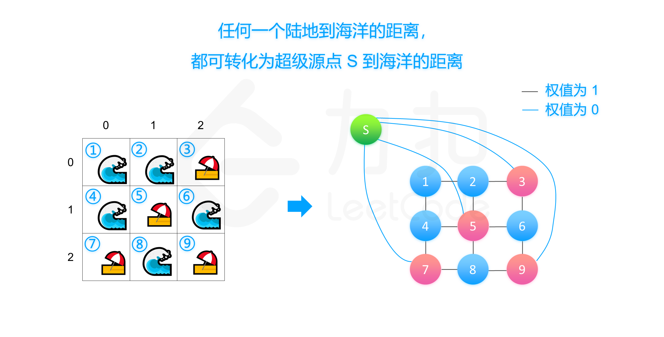
思考:为什么? 因为我们这样做相当于建立了一个超级源点 S,这个点与源点集中的 s_0, s_1, s_2 \cdots s_{|V| 都有边,并且权都为 0。这样求源点集到目标点集的最短路就变成了求超级源点 S 到它们的最短路,于是又转化成了 SSSP 问题。
思考:海洋区域和陆地区域,应该哪一个作为源点集? 也许你分析出「我们需要找一个海洋区域,满足它到陆地的最小距离是最大」会把海洋区域作为源点集。我们可以考虑后续的实现,我们知道 Dijkstra 中一个 d 数组用来维护当前源点集到其他点的最短路,而对于源点集中的任意一个点 s,d[s_x][s_y] = 0,这很好理解,源点到源点的最短路就是 0。如果我们把海洋区域作为源点集、陆地区域作为目标点集,假设 t 是目标点集中的一个点,算法执行结束后 d[t_x][t_y] 就是海洋区域中的点到 t 的最短距离,但是我们却不知道哪些 t 是海洋区域的这些点的「最近陆地区域」,我们也不知道每个 s 距离它的「最近陆地区域」的曼哈顿距离。考虑我们把陆地区域作为源点集、海洋区域作为目标点集,目标点集中的点 t 对应的 d[t_x][t_y] 就是海洋区域 t 对应的距离它的「最近陆地区域」的曼哈顿距离,正是我们需要的,所以应该把陆地区域作为源点集。
最终我们只需要比出 d[t_x][t_y] 的最大值即可。Dijkstra 算法在初始化 d 数组的时候,把每个元素预置为 INF,所以如果发现最终比出的最大值为 INF,那么就返回 -1。
由于这里的边权为 1,也可以直接使用多源 BFS,在这里每个点都只会被松弛一次。
代码实现如下。
代码实现
[sol2-C++] 1 2 3 4 5 6 7 8 9 10 11 12 13 14 15 16 17 18 19 20 21 22 23 24 25 26 27 28 29 30 31 32 33 34 35 36 37 38 39 40 41 42 43 44 45 46 47 48 49 50 51 52 53 54 55 56 57 58 59 60 61 62 63 class Solution {public : static constexpr int MAX_N = 100 + 5 ; static constexpr int INF = int (1E6 ); static constexpr int dx[4 ] = {-1 , 0 , 1 , 0 }, dy[4 ] = {0 , 1 , 0 , -1 }; int n; int d[MAX_N][MAX_N]; struct Status { int v, x, y; bool operator < (const Status &rhs) const { return v > rhs.v; } }; priority_queue <Status> q; int maxDistance (vector<vector<int >>& grid) this ->n = grid.size (); auto &a = grid; for (int i = 0 ; i < n; ++i) { for (int j = 0 ; j < n; ++j) { d[i][j] = INF; } } for (int i = 0 ; i < n; ++i) { for (int j = 0 ; j < n; ++j) { if (a[i][j]) { d[i][j] = 0 ; q.push ({0 , i, j}); } } } while (!q.empty ()) { auto f = q.top (); q.pop (); for (int i = 0 ; i < 4 ; ++i) { int nx = f.x + dx[i], ny = f.y + dy[i]; if (!(nx >= 0 && nx <= n - 1 && ny >= 0 && ny <= n - 1 )) { continue ; } if (f.v + 1 < d[nx][ny]) { d[nx][ny] = f.v + 1 ; q.push ({d[nx][ny], nx, ny}); } } } int ans = -1 ; for (int i = 0 ; i < n; ++i) { for (int j = 0 ; j < n; ++j) { if (!a[i][j]) { ans = max (ans, d[i][j]); } } } return (ans == INF) ? -1 : ans; } };
[sol2-Java] 1 2 3 4 5 6 7 8 9 10 11 12 13 14 15 16 17 18 19 20 21 22 23 24 25 26 27 28 29 30 31 32 33 34 35 36 37 38 39 40 41 42 43 44 45 46 47 48 49 50 51 52 53 54 class Solution { public int maxDistance (int [][] grid) { final int INF = 1000000 ; int [] dx = {-1 , 0 , 1 , 0 }; int [] dy = {0 , 1 , 0 , -1 }; int n = grid.length; int [][] d = new int [n][n]; PriorityQueue<int []> queue = new PriorityQueue <int []>(new Comparator <int []>() { public int compare (int [] status1, int [] status2) { return status1[0 ] - status2[0 ]; } }); for (int i = 0 ; i < n; ++i) { for (int j = 0 ; j < n; ++j) { d[i][j] = INF; } } for (int i = 0 ; i < n; ++i) { for (int j = 0 ; j < n; ++j) { if (grid[i][j] == 1 ) { d[i][j] = 0 ; queue.offer(new int []{0 , i, j}); } } } while (!queue.isEmpty()) { int [] f = queue.poll(); for (int i = 0 ; i < 4 ; ++i) { int nx = f[1 ] + dx[i], ny = f[2 ] + dy[i]; if (!(nx >= 0 && nx < n && ny >= 0 && ny < n)) { continue ; } if (f[0 ] + 1 < d[nx][ny]) { d[nx][ny] = f[0 ] + 1 ; queue.offer(new int []{d[nx][ny], nx, ny}); } } } int ans = -1 ; for (int i = 0 ; i < n; ++i) { for (int j = 0 ; j < n; ++j) { if (grid[i][j] == 0 ) { ans = Math.max(ans, d[i][j]); } } } return ans == INF ? -1 : ans; } }
[sol2-C++] 1 2 3 4 5 6 7 8 9 10 11 12 13 14 15 16 17 18 19 20 21 22 23 24 25 26 27 28 29 30 31 32 33 34 35 36 37 38 39 40 41 42 43 44 45 46 47 48 49 50 51 52 53 54 55 56 57 58 class Solution {public : static constexpr int MAX_N = 100 + 5 ; static constexpr int INF = int (1E6 ); static constexpr int dx[4 ] = {-1 , 0 , 1 , 0 }, dy[4 ] = {0 , 1 , 0 , -1 }; int n; int d[MAX_N][MAX_N]; struct Coordinate { int x, y; }; queue <Coordinate> q; int maxDistance (vector<vector<int >>& grid) this ->n = grid.size (); auto &a = grid; for (int i = 0 ; i < n; ++i) { for (int j = 0 ; j < n; ++j) { d[i][j] = INF; } } for (int i = 0 ; i < n; ++i) { for (int j = 0 ; j < n; ++j) { if (a[i][j]) { d[i][j] = 0 ; q.push ({i, j}); } } } while (!q.empty ()) { auto f = q.front (); q.pop (); for (int i = 0 ; i < 4 ; ++i) { int nx = f.x + dx[i], ny = f.y + dy[i]; if (!(nx >= 0 && nx <= n - 1 && ny >= 0 && ny <= n - 1 )) continue ; if (d[nx][ny] > d[f.x][f.y] + 1 ) { d[nx][ny] = d[f.x][f.y] + 1 ; q.push ({nx, ny}); } } } int ans = -1 ; for (int i = 0 ; i < n; ++i) { for (int j = 0 ; j < n; ++j) { if (!a[i][j]) { ans = max (ans, d[i][j]); } } } return (ans == INF) ? -1 : ans; } };
[sol2-Java] 1 2 3 4 5 6 7 8 9 10 11 12 13 14 15 16 17 18 19 20 21 22 23 24 25 26 27 28 29 30 31 32 33 34 35 36 37 38 39 40 41 42 43 44 45 46 47 48 49 50 class Solution { public int maxDistance (int [][] grid) { final int INF = 1000000 ; int [] dx = {-1 , 0 , 1 , 0 }; int [] dy = {0 , 1 , 0 , -1 }; int n = grid.length; int [][] d = new int [n][n]; Queue<int []> queue = new LinkedList <int []>(); for (int i = 0 ; i < n; ++i) { for (int j = 0 ; j < n; ++j) { d[i][j] = INF; } } for (int i = 0 ; i < n; ++i) { for (int j = 0 ; j < n; ++j) { if (grid[i][j] == 1 ) { d[i][j] = 0 ; queue.offer(new int []{i, j}); } } } while (!queue.isEmpty()) { int [] f = queue.poll(); for (int i = 0 ; i < 4 ; ++i) { int nx = f[0 ] + dx[i], ny = f[1 ] + dy[i]; if (!(nx >= 0 && nx < n && ny >= 0 && ny < n)) { continue ; } if (d[nx][ny] > d[f[0 ]][f[1 ]] + 1 ) { d[nx][ny] = d[f[0 ]][f[1 ]] + 1 ; queue.offer(new int []{nx, ny}); } } } int ans = -1 ; for (int i = 0 ; i < n; ++i) { for (int j = 0 ; j < n; ++j) { if (grid[i][j] == 0 ) { ans = Math.max(ans, d[i][j]); } } } return ans == INF ? -1 : ans; } }
[sol2-C++] 1 2 3 4 5 6 7 8 9 10 11 12 13 14 15 16 17 18 19 20 21 22 23 24 25 26 27 28 29 30 31 32 33 34 35 36 37 38 39 40 41 42 43 44 45 46 47 48 49 50 51 52 53 54 55 56 57 58 59 60 61 62 63 64 65 class Solution {public : static constexpr int MAX_N = 100 + 5 ; static constexpr int INF = int (1E6 ); static constexpr int dx[4 ] = {-1 , 0 , 1 , 0 }, dy[4 ] = {0 , 1 , 0 , -1 }; int n; int d[MAX_N][MAX_N]; struct Coordinate { int x, y; }; queue <Coordinate> q; bool inq[MAX_N][MAX_N]; int maxDistance (vector<vector<int >>& grid) this ->n = grid.size (); auto &a = grid; for (int i = 0 ; i < n; ++i) { for (int j = 0 ; j < n; ++j) { d[i][j] = INF; } } for (int i = 0 ; i < n; ++i) { for (int j = 0 ; j < n; ++j) { if (a[i][j]) { d[i][j] = 0 ; q.push ({i, j}); inq[i][j] = 1 ; } } } while (!q.empty ()) { auto f = q.front (); q.pop (); inq[f.x][f.y] = 0 ; for (int i = 0 ; i < 4 ; ++i) { int nx = f.x + dx[i], ny = f.y + dy[i]; if (!(nx >= 0 && nx <= n - 1 && ny >= 0 && ny <= n - 1 )) { continue ; } if (d[nx][ny] > d[f.x][f.y] + 1 ) { d[nx][ny] = d[f.x][f.y] + 1 ; if (!inq[nx][ny]) { q.push ({nx, ny}); inq[nx][ny] = 1 ; } } } } int ans = -1 ; for (int i = 0 ; i < n; ++i) { for (int j = 0 ; j < n; ++j) { if (!a[i][j]) { ans = max (ans, d[i][j]); } } } return (ans == INF) ? -1 : ans; } };
[sol2-Java] 1 2 3 4 5 6 7 8 9 10 11 12 13 14 15 16 17 18 19 20 21 22 23 24 25 26 27 28 29 30 31 32 33 34 35 36 37 38 39 40 41 42 43 44 45 46 47 48 49 50 51 52 53 54 55 56 class Solution { public int maxDistance (int [][] grid) { final int INF = 1000000 ; int [] dx = {-1 , 0 , 1 , 0 }; int [] dy = {0 , 1 , 0 , -1 }; int n = grid.length; int [][] d = new int [n][n]; Queue<int []> queue = new LinkedList <int []>(); boolean [][] inq = new boolean [n][n]; for (int i = 0 ; i < n; ++i) { for (int j = 0 ; j < n; ++j) { d[i][j] = INF; } } for (int i = 0 ; i < n; ++i) { for (int j = 0 ; j < n; ++j) { if (grid[i][j] == 1 ) { d[i][j] = 0 ; queue.offer(new int []{i, j}); inq[i][j] = true ; } } } while (!queue.isEmpty()) { int [] f = queue.poll(); inq[f[0 ]][f[1 ]] = false ; for (int i = 0 ; i < 4 ; ++i) { int nx = f[0 ] + dx[i], ny = f[1 ] + dy[i]; if (!(nx >= 0 && nx < n && ny >= 0 && ny < n)) { continue ; } if (d[nx][ny] > d[f[0 ]][f[1 ]] + 1 ) { d[nx][ny] = d[f[0 ]][f[1 ]] + 1 ; if (!inq[nx][ny]) { queue.offer(new int []{nx, ny}); inq[nx][ny] = true ; } } } } int ans = -1 ; for (int i = 0 ; i < n; ++i) { for (int j = 0 ; j < n; ++j) { if (grid[i][j] == 0 ) { ans = Math.max(ans, d[i][j]); } } } return ans == INF ? -1 : ans; } }
复杂度分析
时间复杂度:考虑这里的「多源最短路」的本质还是「单源最短路」,因此就是 Dijkstra 算法堆优化版本的渐进时间复杂度 O(E \log V),这里 E 为边的个数,约等于 4n^2/2,V 为顶点个数,约等于 n^2,所以这里的渐进时间复杂度为 O(n^2 \log n^2) = O(n^2 \log n);在多源 BFS 当中,由于每个点只能被访问一次,渐进时间复杂度为 O(V+E) = O(n^2);SPFA 算法的理论渐进上界是 O(VE) = O(n^2),但是由于这里的边权都为 1,于是它退化成了 BFS,渐进时间复杂度 O(n^2)。
空间复杂度:该算法使用了 d 数组,渐进空间复杂度为 O(n^2)。
方法三:动态规划 思路
考虑优化方法二中的「把陆地区域作为源点集、海洋区域作为目标点集,求最短路」的过程。我们知道对于每个海洋区域 (x, y),离它最近的陆地区域到它的路径要么从上方或者左方来,要么从右方或者下方来。考虑做两次动态规划,第一次从左上到右下,第二次从右下到左上,记 f(x, y) 为 (x, y) 距离最近的陆地区域的曼哈顿距离,则我们可以推出这样的转移方程:
f(x, y) = \left { \begin{aligned} & 0 & , & (x, y) {\rm , is, land} \ & \min { f(x - 1, y), f(x, y - 1) } + 1 & , & (x, y) {\rm , is,ocean} \end{aligned} \right.
f(x, y) = \left { \begin{aligned} & 0 & , & (x, y) {\rm , is, land} \ & \min { f(x + 1, y), f(x, y + 1) } + 1 & , & (x, y) {\rm , is,ocean} \end{aligned} \right.
我们初始化的时候把陆地的 f 值全部预置为 0,海洋的 f 全部预置为 INF,做完两个阶段的动态规划后,我们在所有的不为零的 f[i][j] 中比一个最大值即可,如果最终比较出的最大值为 INF,就返回 -1。
思考:如果用 f(x, y) 记录左上方的 DP 结果,g(x, y) 记录右下方的DP结果可行吗? 答案是不可行。因为考虑距离点 (x, y) 最近的点可能既不来自左上方,也不来自右下方,比如它来自右上方,这个时候,第二阶段我们就需要用到第一阶段的计算结果。
代码实现如下。
代码实现
[sol3-C++] 1 2 3 4 5 6 7 8 9 10 11 12 13 14 15 16 17 18 19 20 21 22 23 24 25 26 27 28 29 30 31 32 33 34 35 36 37 38 39 40 41 42 43 44 45 46 47 48 49 50 51 52 53 54 55 56 57 58 59 60 61 62 class Solution {public : static constexpr int MAX_N = 100 + 5 ; static constexpr int INF = int (1E6 ); int f[MAX_N][MAX_N]; int n; int maxDistance (vector<vector<int >>& grid) this ->n = grid.size (); vector<vector<int >>& a = grid; for (int i = 0 ; i < n; ++i) { for (int j = 0 ; j < n; ++j) { f[i][j] = (a[i][j] ? 0 : INF); } } for (int i = 0 ; i < n; ++i) { for (int j = 0 ; j < n; ++j) { if (a[i][j]) { continue ; } if (i - 1 >= 0 ) { f[i][j] = min (f[i][j], f[i - 1 ][j] + 1 ); } if (j - 1 >= 0 ) { f[i][j] = min (f[i][j], f[i][j - 1 ] + 1 ); } } } for (int i = n - 1 ; i >= 0 ; --i) { for (int j = n - 1 ; j >= 0 ; --j) { if (a[i][j]) { continue ; } if (i + 1 < n) { f[i][j] = min (f[i][j], f[i + 1 ][j] + 1 ); } if (j + 1 < n) { f[i][j] = min (f[i][j], f[i][j + 1 ] + 1 ); } } } int ans = -1 ; for (int i = 0 ; i < n; ++i) { for (int j = 0 ; j < n; ++j) { if (!a[i][j]) { ans = max (ans, f[i][j]); } } } if (ans == INF) { return -1 ; } else { return ans; } } };
[sol3-Java] 1 2 3 4 5 6 7 8 9 10 11 12 13 14 15 16 17 18 19 20 21 22 23 24 25 26 27 28 29 30 31 32 33 34 35 36 37 38 39 40 41 42 43 44 45 46 47 48 49 50 51 52 53 54 55 class Solution { public int maxDistance (int [][] grid) { final int INF = 1000000 ; int n = grid.length; int [][] f = new int [n][n]; for (int i = 0 ; i < n; ++i) { for (int j = 0 ; j < n; ++j) { f[i][j] = grid[i][j] == 1 ? 0 : INF; } } for (int i = 0 ; i < n; ++i) { for (int j = 0 ; j < n; ++j) { if (grid[i][j] == 1 ) { continue ; } if (i - 1 >= 0 ) { f[i][j] = Math.min(f[i][j], f[i - 1 ][j] + 1 ); } if (j - 1 >= 0 ) { f[i][j] = Math.min(f[i][j], f[i][j - 1 ] + 1 ); } } } for (int i = n - 1 ; i >= 0 ; --i) { for (int j = n - 1 ; j >= 0 ; --j) { if (grid[i][j] == 1 ) { continue ; } if (i + 1 < n) { f[i][j] = Math.min(f[i][j], f[i + 1 ][j] + 1 ); } if (j + 1 < n) { f[i][j] = Math.min(f[i][j], f[i][j + 1 ] + 1 ); } } } int ans = -1 ; for (int i = 0 ; i < n; ++i) { for (int j = 0 ; j < n; ++j) { if (grid[i][j] == 0 ) { ans = Math.max(ans, f[i][j]); } } } if (ans == INF) { return -1 ; } else { return ans; } } }
复杂度分析